- The link between prediction and accomplishment. A math theory develops in
several stages. Each stage has its own technical language. Each book can focus
on one single language. Few people can understand all the stages of development.
A great accomplishment comes from a brave prediction [Bir, p.56, l.1]. We should
identify the vital link between prediction and accomplishment. If we fail to
rigorously prove our conjecture, then our plan will never be fulfilled. If we
generalize something without knowing its origin, then the generalization has no
primitive model to follow. In order to fully understand a theory's
development, we need clear references to exactly match an accomplishment with
its corresponding prediction. Example 1. [Bir, p.55, (42) & (44)] predict [Ru3,
pp.192-193, (2) & (4)].
It is not enough to prove the given answer is correct. We would like to know
where the answer comes from in the first place. Example 2. [Bir, p.47, (29);
p.48, (30)] predict [Bir, p. 48, Theorem 8]. Namely, the Green function in [Bir,
p.48, Theorem 8] originates from impulsive initial velocity [Bir, p.46, l.9].
Significant theories come directly from experiments. It is indispensable that
Birkhoff gives a reference [Bir, p.53, l.-2] to show how to build a solution
from scratch [Gri, p.92, l.-9-p.93, l.20]. If he had
just given the solution from nowhere, we would have to say that his solution in
[Bir, p.54, Theorem 10] is neither effective nor complete. In other words, if
Birkhoff had omitted [Bir, p.53, l.3-l.21], we never could have figured out the
origin of f & g in [Bir, p.53, l.- 6].
- The link between a key concept and its applications. Green's
functions play important roles in variation of parameters and distribution
theory. In order to fully understand what we have learned, we must link these
packages together and build our math network. [Bir, chap.2,
§9 & p.55, Delta-function
Interpretation]
- The link between the corresponding landmark statements.
We may approach the same goal by two different methods. During the process
there are some equivalent landmark statements that can be interpreted with
respect to the corresponding methods. The link between the equivalent landmarks
has only a shallow meaning on its own, but it has a deep meaning if we have our
original goal in mind.
[Arn, §25.1] gives two methods to
calculate eAt. We would like to interpret
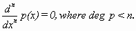
Δn=0 [Arn, p.168, l.-3] in terms
of the differential operator. If l =0 in A [Arn,
p.167, l.15], then A=Δ.
Δn=0 means
- Systematizing the inputs from various perspectives.
We may discuss variation of constants in various perspectives. [Bir, p.48,
Example 6] gives the origin of Green's
function and predicts the exact formula of the solution. [Arn, p.210, Remark]
provides a practical method. [Arn, p.208, l.-
3-p.209, l.10] summarizes the argument with a simple strategy. In some sense
these input images are one. We would like to systematize them and choose the
most convenient solution form that can easily conjure up all the above images.
- Interact with the theme.
To solve a problem, we would like to find a solution which may somehow
interact with the problem's
geometrical and physical interpretation [Volumes, phase flow; Arn, p.196, l.-19-l.-3]. The key idea obtained by this method may
not only solve the case in point, but may also have an importance on a stronger
case [Arn, p.198, l.14]. In [Har, p.47, l.1-l.9], Hartman juggles with mechanic
properties that have nothing to do with the geometrical or physical meaning of
the problem. [Inc, p.175] executes the step-by-step calculation by following
Hartman's method.
- The link between a method and its applications.
[Har, p.50, Lemma 3.1] shows that we may use reduction of order to find all
the solutions of a linear DE locally [Har, p.49, l.-10]. [Inc, p.103, §38] fail to list
important applications. [Inc, p.111, (42.3); p.155, l.6] and [Bir, p.242, l.18]
fail to remind readers that reduction of order justifies the substitution [Har,
p.327, l.14-l.17].
- We should avoid repetition and reduce the entire theory to its hard core.
- Inseparability of a theorem from its role in the entire
theory.
We like to isolate certain facts from a context and give them the status of a
theorem. In doing so, we often ignore the inseparability of a theorem from the
role it plays in the entire theory.
For the application of a theorem, we would like to study how often it appears
in the theory, in which areas it appears, and in what form it fits into its
surroundings.
Example. Let us compare how [Joh, p.153, l.8] and [Ru3, p.180, l.10]
introduce the Paley-Wiener theorem into the theory of PDE.
- We may use Green's functions,
integral transforms, or separation of variables to solve PDE's
[Sne, chap.3]. However, these methods are closely related. More precisely, each
method leads to the next one.
We need Green's function to
solve [Sne, p.294, (1),(2),(3)].
® We use the Laplace transform to determine Green's
function [Sne, p.297, l.2].
® In view of [Sne, p.298, (16)], we may also use separation of
variables [Sne, p.298, l.6].
- Go to the basics to establish the main relationship.
- The lack of development may make us mistake a partial aspect for the big
picture.
The way Goldstein uses the inertia tensor may make his readers believe that
tensors and linear transformations are the same [Gol, p.147, l.14-l.29]. In
fact, this viewpoint can be justified only under certain conditions [War, p.55,
(d)].
Note. [Gol, p.146, (5-9)] is a corollary of [War, p.55, (e)].
- The relationship between the basic concepts (the tensor algebra and the
exterior algebra) can be fully established [War, p.56, Definition 2.4].
The tensor product and wedge product in [War, pp. 54-65] establish the
relationships among three isolated major treatments: Lang's
algebraic treatment [Lan, chap. XVI], Goldstein's
treatment for mechanics [Gol, p.146, l.15-p.147, l.-8], and Spivak's superficial treatment
for differential geometry [Spi, vol.1, chap. 4 & chap. 7].
- The domains of the tensor product and the wedge product are fully
developed.
- The operations become simple and direct. Example (tensor product):
Compare [War, p.54, Definition 2.1] with [Spi, vol.1, p.159, l.7].
- The artificial outlook of synthetic properties can be illustrated by
basic inner operations.
Compare [War, p.56, Definition 2.4; p.57, 2.6(a)] with [O'N,
p.153, l.-1].
- (Inclusiveness and consistency)
The scheme in [War, pp.54-62, §2.1-§2.13] is consistent with almost every existing concept of product.
- Multiplication of real numbers [War, p.59, l.14].
- Scalar product [Arn2, p.173, Problem 7].
- Vector product [Arn2, p.173, Problem 6].
- (Lie group with its Lie algebra)
Quaternion product = vector product - scalar
product [Po3, p.170, l.1].
Bracket product = vector product [Po3, p.384, Example 93].
- (Sorting)
We would like to distinguish between the identification by general properties
(the 2nd isomorphism in [War, p.60, l.2]) and the identification by a particular
assignment (the 1st isomorphism in [War, p.60, l.2]). Only for the latter may we
have the freedom to make a choice for adjustment [War, p.60, l.5].
- The basics are developed through research experiences that provide
clarification. Most common mistakes committed by mathematicians are basics.
These basics may look confusing unless they are well-isolated from complicated
situations.
- The basics are the foundation in building and expanding a theory. They
are constantly modified by experimental results in order to advance further
research.
- One topic cannot be completed without the other [Mas, p.145, l.-18-l.-13].
- A scheme for the implication diagram.
We use the following strategy to build a tight and economical network:
- If both AÞ B and BÞ
A are true, then we write A iff B. If we write AÞ B,
it means that BÞ A is false [Dug, p.311, l.-
8].
- If AÞ C and BÞ C
both appear in the diagram, then it means that both AÞ
B and BÞ A are false [Dug, p.311, Diagram; p.238,
l.3; p.239, Ex.2].
Remark 1. The proof in [Po3, p.69, Example 24] is unnecessary because we can
derive it more quickly from the diagram in [Dug, p.311].
Remark 2. The path "Compact Þ
s-compact Þ Regular Lindelöf
Þ Paracompact Þ Normal"
[Dug, p.311, Diagram] is a detour. There is a simple and direct proof in [Per,
p.91, Theorem 5.5.5].
- How a math network strengthens effectiveness.
(Identification of fundamental groups)
- Product [Po3, p.350, F)].
- Homomorphic image [Po3, p.370, l.-7]. A
covering space is a generalization of a topological group homomorphism [Po3,
p.134, C)]. The use of universal coverings makes it easy to identify the
fundamental group of a homomorphic image.
- Although we can define the fundamental group in an arcwise connected
topological space R [Po3, p.348, Definition 44], for its identification we often
wonder where to start if R does not have any group structure.
Remarks from the viewpoint of a math network. [Mas] completely ignores the
role of topological group homomorphisms when discussing covering spaces. [Po3]
shows the complete development process: Topological group homomorphism
® covering space ®
covering group. Imposing a group structure on a covering space is like
going back to the original stage. [War] lacks the first part of the development
(Topological group homomorphisms ® covering space).
- The correct approach toward developing a theory is to use the important
facts as milestones and then link these facts with theorems. In contrast, the
incorrect approach is to use the big theorems as the milestones and
link them with examples.
In [Cou2, vol. 1, p.359], the evolute E of a curve C is defined as the locus of the centers of curvature of C.
In [Cou2, vol. 2, p.301, l.5], the evolute E of a curve C is defined as the
envelope of the normals of C. In [Cou2, vol. 1, p.424], Courant proves that the
first definition implies the second one. In [Cou2, vol. 2, p.301, Example 11],
Courant proves that the second definition implies the first one. [Wea1, vol.
1, §10 & §11]
discuss involutes and evolutes, but fail to link evolutes with the concept of
centers of curvature.
- A physicist may be familiar with the discussion given in [Jack,
§3.4], but may not be able to prove the statement given in [Jack, p.105, l.12-l.13]. A mathematician may understand the proof of [Guo, p.214, (12)], but may not understand the story given in [Jack,
§3.4]. In order to fully understand the formula given in [Guo, p.214, (12)], one
must understand both its mathematical meaning and physical applications.
- Gauss, Lagrange, Kummer, and Hilbert wrote important work after mastering mathematics and physics.
Their deep understanding of mathematical network enabled them to write
masterpieces. It would be difficult to do so for those who specialize only a
narrow field. Galois was able to write great work because he had read Lagrange's
opus. Einstein had also read many people's work before he wrote papers on
relativity. Mastering mathematical networks may help us deduce simplicity from
apparent complicity, recognize the essence, understand the situation, propose
important questions, and write significant papers.
- Recognizing a theorem's attributes helps find its proof and determine the role that it plays in a theory.
From the viewpoint of Hartman, [Har, p.14, Corollary 3.1] and [Har, p.14, Corollary 3.2] are corollaries of [Har,
pp.12-13, Theorem 3.1] because it is necessary to prove the existence of a
maximum interval before discussing it. In my opinion, the two corollaries and the theorem are corollaries of [Har, p.11, Corollary 2.1] because the key idea of the proofs of the former tree is [Har, p.11, Corollary 2.1].
- A theorem with added features
A pizza with sausage topping is still a pizza,; it will not become a stake. [Har, pp.14-15, Theorem 3.2] is a generalization of [Har, pp.4-5, Theorem 2.4] with the feature of maximum iterval.
[Har, pp.12-13, Theorem 3.1] shows the existence of a maximum interval. Consequently, the proof of [Har, pp.14-15, Theorem 3.2] is the proof of [Har, pp.4-5, Theorem 2.4] plus that of [Har, pp.12-13, Theorem 3.1], and nothing else. If we fail to relate [Har, pp.14-15, Theorem 3.2] to other theorems, its proof could look quite complicated.
- The scope of a method's applicability
When a method is related to a problem, we should apply the method to
only where it may, and leave the rest to be dealt with in another way. In a finite-dimensional normed space, its various product norms are equivalent [Ru3, pp-14-15, §1.19]. Consequently, all the properties of finite-dimensional normed spaces remain valid if we replace one product norm with another. However, we cannot use this method to prove that [Har, p.26, Lemma 3.2] implies [Har, p.26, Exercise 3.1]. Instead, we should prove the latter statement as follows:
Proof. Let h>0.
lim h®0(|yj(t+h)|-|yj(t)|)/h = yj'(t) sgn yj(t) (j = 1,…,d)
[Har, p.26, Lemma 3.1].
lim h®0(|y1(t+h)|-|y1(t)|,…,|yd(t+h)|-|yd(t)|)/h = (y1'(t) sgn y1(t),…,yd'(t) sgn yd(t)).
Taking the Euclidean norm on both sides, we have DR|y(t)|=|y'(t)|.
It is not enough to prove the given answer is correct. We would like to know where the answer comes from in the first place. Example 2. [Bir, p.47, (29); p.48, (30)] predict [Bir, p. 48, Theorem 8]. Namely, the Green function in [Bir, p.48, Theorem 8] originates from impulsive initial velocity [Bir, p.46, l.9].
Significant theories come directly from experiments. It is indispensable that Birkhoff gives a reference [Bir, p.53, l.-2] to show how to build a solution from scratch [Gri, p.92, l.-9-p.93, l.20]. If he had just given the solution from nowhere, we would have to say that his solution in [Bir, p.54, Theorem 10] is neither effective nor complete. In other words, if Birkhoff had omitted [Bir, p.53, l.3-l.21], we never could have figured out the origin of f & g in [Bir, p.53, l.- 6].
We may approach the same goal by two different methods. During the process there are some equivalent landmark statements that can be interpreted with respect to the corresponding methods. The link between the equivalent landmarks has only a shallow meaning on its own, but it has a deep meaning if we have our original goal in mind.
[Arn, §25.1] gives two methods to calculate eAt. We would like to interpret Δn=0 [Arn, p.168, l.-3] in terms of the differential operator. If l =0 in A [Arn, p.167, l.15], then A=Δ. Δn=0 means
![]()
We may discuss variation of constants in various perspectives. [Bir, p.48, Example 6] gives the origin of Green's function and predicts the exact formula of the solution. [Arn, p.210, Remark] provides a practical method. [Arn, p.208, l.- 3-p.209, l.10] summarizes the argument with a simple strategy. In some sense these input images are one. We would like to systematize them and choose the most convenient solution form that can easily conjure up all the above images.
To solve a problem, we would like to find a solution which may somehow interact with the problem's geometrical and physical interpretation [Volumes, phase flow; Arn, p.196, l.-19-l.-3]. The key idea obtained by this method may not only solve the case in point, but may also have an importance on a stronger case [Arn, p.198, l.14]. In [Har, p.47, l.1-l.9], Hartman juggles with mechanic properties that have nothing to do with the geometrical or physical meaning of the problem. [Inc, p.175] executes the step-by-step calculation by following Hartman's method.
[Har, p.50, Lemma 3.1] shows that we may use reduction of order to find all the solutions of a linear DE locally [Har, p.49, l.-10]. [Inc, p.103, §38] fail to list important applications. [Inc, p.111, (42.3); p.155, l.6] and [Bir, p.242, l.18] fail to remind readers that reduction of order justifies the substitution [Har, p.327, l.14-l.17].
We like to isolate certain facts from a context and give them the status of a theorem. In doing so, we often ignore the inseparability of a theorem from the role it plays in the entire theory.
For the application of a theorem, we would like to study how often it appears in the theory, in which areas it appears, and in what form it fits into its surroundings.
Example. Let us compare how [Joh, p.153, l.8] and [Ru3, p.180, l.10] introduce the Paley-Wiener theorem into the theory of PDE.
We need Green's function to solve [Sne, p.294, (1),(2),(3)].
® We use the Laplace transform to determine Green's function [Sne, p.297, l.2].
® In view of [Sne, p.298, (16)], we may also use separation of variables [Sne, p.298, l.6].
- The lack of development may make us mistake a partial aspect for the big
picture.
The way Goldstein uses the inertia tensor may make his readers believe that tensors and linear transformations are the same [Gol, p.147, l.14-l.29]. In fact, this viewpoint can be justified only under certain conditions [War, p.55, (d)].
Note. [Gol, p.146, (5-9)] is a corollary of [War, p.55, (e)]. - The relationship between the basic concepts (the tensor algebra and the
exterior algebra) can be fully established [War, p.56, Definition 2.4].
The tensor product and wedge product in [War, pp. 54-65] establish the relationships among three isolated major treatments: Lang's algebraic treatment [Lan, chap. XVI], Goldstein's treatment for mechanics [Gol, p.146, l.15-p.147, l.-8], and Spivak's superficial treatment for differential geometry [Spi, vol.1, chap. 4 & chap. 7].- The domains of the tensor product and the wedge product are fully developed.
- The operations become simple and direct. Example (tensor product): Compare [War, p.54, Definition 2.1] with [Spi, vol.1, p.159, l.7].
- The artificial outlook of synthetic properties can be illustrated by
basic inner operations.
Compare [War, p.56, Definition 2.4; p.57, 2.6(a)] with [O'N, p.153, l.-1].
- (Inclusiveness and consistency)
The scheme in [War, pp.54-62, §2.1-§2.13] is consistent with almost every existing concept of product.- Multiplication of real numbers [War, p.59, l.14].
- Scalar product [Arn2, p.173, Problem 7].
- Vector product [Arn2, p.173, Problem 6].
- (Lie group with its Lie algebra)
Quaternion product = vector product - scalar product [Po3, p.170, l.1].
Bracket product = vector product [Po3, p.384, Example 93].
- (Sorting)
We would like to distinguish between the identification by general properties (the 2nd isomorphism in [War, p.60, l.2]) and the identification by a particular assignment (the 1st isomorphism in [War, p.60, l.2]). Only for the latter may we have the freedom to make a choice for adjustment [War, p.60, l.5]. - The basics are developed through research experiences that provide clarification. Most common mistakes committed by mathematicians are basics. These basics may look confusing unless they are well-isolated from complicated situations.
- The basics are the foundation in building and expanding a theory. They are constantly modified by experimental results in order to advance further research.
We use the following strategy to build a tight and economical network:
- If both AÞ B and BÞ A are true, then we write A iff B. If we write AÞ B, it means that BÞ A is false [Dug, p.311, l.- 8].
- If AÞ C and BÞ C both appear in the diagram, then it means that both AÞ B and BÞ A are false [Dug, p.311, Diagram; p.238, l.3; p.239, Ex.2].
Remark 2. The path "Compact Þ s-compact Þ Regular Lindelöf Þ Paracompact Þ Normal" [Dug, p.311, Diagram] is a detour. There is a simple and direct proof in [Per, p.91, Theorem 5.5.5].
(Identification of fundamental groups)
- Product [Po3, p.350, F)].
- Homomorphic image [Po3, p.370, l.-7]. A covering space is a generalization of a topological group homomorphism [Po3, p.134, C)]. The use of universal coverings makes it easy to identify the fundamental group of a homomorphic image.
- Although we can define the fundamental group in an arcwise connected topological space R [Po3, p.348, Definition 44], for its identification we often wonder where to start if R does not have any group structure.
In [Cou2, vol. 1, p.359], the evolute E of a curve C is defined as the locus of the centers of curvature of C. In [Cou2, vol. 2, p.301, l.5], the evolute E of a curve C is defined as the envelope of the normals of C. In [Cou2, vol. 1, p.424], Courant proves that the first definition implies the second one. In [Cou2, vol. 2, p.301, Example 11], Courant proves that the second definition implies the first one. [Wea1, vol. 1, §10 & §11] discuss involutes and evolutes, but fail to link evolutes with the concept of centers of curvature.
- Recognizing a theorem's attributes helps find its proof and determine the role that it plays in a theory.
From the viewpoint of Hartman, [Har, p.14, Corollary 3.1] and [Har, p.14, Corollary 3.2] are corollaries of [Har, pp.12-13, Theorem 3.1] because it is necessary to prove the existence of a maximum interval before discussing it. In my opinion, the two corollaries and the theorem are corollaries of [Har, p.11, Corollary 2.1] because the key idea of the proofs of the former tree is [Har, p.11, Corollary 2.1]. - A theorem with added features
A pizza with sausage topping is still a pizza,; it will not become a stake. [Har, pp.14-15, Theorem 3.2] is a generalization of [Har, pp.4-5, Theorem 2.4] with the feature of maximum iterval. [Har, pp.12-13, Theorem 3.1] shows the existence of a maximum interval. Consequently, the proof of [Har, pp.14-15, Theorem 3.2] is the proof of [Har, pp.4-5, Theorem 2.4] plus that of [Har, pp.12-13, Theorem 3.1], and nothing else. If we fail to relate [Har, pp.14-15, Theorem 3.2] to other theorems, its proof could look quite complicated.
When a method is related to a problem, we should apply the method to only where it may, and leave the rest to be dealt with in another way. In a finite-dimensional normed space, its various product norms are equivalent [Ru3, pp-14-15, §1.19]. Consequently, all the properties of finite-dimensional normed spaces remain valid if we replace one product norm with another. However, we cannot use this method to prove that [Har, p.26, Lemma 3.2] implies [Har, p.26, Exercise 3.1]. Instead, we should prove the latter statement as follows:
Proof. Let h>0.
lim h®0(|yj(t+h)|-|yj(t)|)/h = yj'(t) sgn yj(t) (j = 1,…,d) [Har, p.26, Lemma 3.1].
lim h®0(|y1(t+h)|-|y1(t)|,…,|yd(t+h)|-|yd(t)|)/h = (y1'(t) sgn y1(t),…,yd'(t) sgn yd(t)).
Taking the Euclidean norm on both sides, we have DR|y(t)|=|y'(t)|.