D.N. Meehan*, Union Pacific Resources Co, and S.K. Verma,* Stanford U.
* SPE Members
Copyright 1994, Society of Petroleum Engineers, Inc.
This paper was prepared for presentation at the SPE 69th Annual Technical Conference and Exhibition held in New Orleans, LA. USA, 25-28 September 1994.
This paper was selected for presentation
by an SPE Program Committee following review of information contained
in an abstract submitted by the author(s). Contents of the paper,
as presented, have not been reviewed by the Society of Petroleum
Engineers and are subject to correction by the author(s). The
material, as presented, does not necessarily reflect any position
of the Society of Petroleum Engineers, its officers, or members.
Papers presented at SPE meetings are subject to publication review
by Editorial Committees of the Society of Petroleum Engineers.
Electronic reproduction, distribution, or storage of any part
of this paper for commercial purposes without the written consent
of the Society of Petroleum Engineers is prohibited. Permission
to reproduce in print is restricted to an abstract of not more
than 300 words; illustrations may not be copied. The abstract
must contain conspicuous acknowledgment of where and by whom the
paper was presented. Write Librarian, SPE, P.O. Box 833836, Richardson,
TX 75083-3836, U.S.A., fax 01-972-952-9435.
Introduction
Infill drilling has been commercially successful
in many low permeability, heterogeneous gas reservoirs. Reservoir
discontinuities have often been suspected as a factor in poor
gas recoveries on wide spacing. Large vertical and lateral variations
in permeability make it difficult to account for partial drainage
at infill locations. How many wells must be drilled to recover
the gas? What are the effects of heterogeneities on optimal well
spacing and fracture length?
In this paper, a case history illustrates the
power of incorporating high resolution, fine grid geostatistical
models in simulating reservoir behavior. Previous reservoir simulation
studies provided acceptable matches of flow rates and pressures
by fairly arbitrary reductions in the log derived net pay for
the entire reservoir or away from the well. However, these models
failed to match extended pressure buildups. The buildups indicate
significantly higher gas-in-place in the reservoir
than is indicated by simulation matches based on simpler reservoir
descriptions. The geostatistical model presented here resulted
in excellent multiple well history matches and matched
the long term buildup.
The techniques for generating the reservoir
description are summarized along with the reservoir simulation
results. Predictions of infill drilling success with this model
are better than for prior models. Predictions of incremental gas
recoveries from infill drilling from this model are consistent
with observed results. Reservoir heterogeneities (specifically
the lateral continuity of permeability) appear to be the most
important factors in this reservoir controlling inadequate drainage
of the uppermost intervals. These lateral heterogeneities appear
to be diagenetic permeability alterations resulting in partial
compartmentalization of the many individual sands.
Optimal well spacing in very low permeability
reservoirs has been addressed by numerous authors. Wells with
permeabilities in the Cotton Valley range (# 0.01 md) generally
indicate extremely long "optimal" fracture lengths (often
in excess of 1000 ft fracture half-lengths). It is doubtful
that such fractures can be created without vastly larger jobs
than predicted by conventional hydraulic fracture models. Economic
approaches used in conventional fracture optimization models may
be inappropriate in thick intervals with few stress barriers.
Inadequate barriers to fracture height growth and reservoir heterogeneities
indicate the need for closer spacing and moderate fracture lengths.
Continued infill drilling accomplishes two
things, viz. increased access to poorly drained portions
of the reservoir with better stimulations and acceleration of
recoveries from the most continuous portions of the reservoir.
Current well costs can justify incremental recoveries at the
current spacing levels; however, significant gas will remain unrecovered.
The importance of lowering well costs is described.
The Carthage (Cotton Valley) Field is located
in Panola County in East Texas. The Cotton Valley sandstones of
Carthage field consist of a series of marine and lagoonal deposits
overlying the gentle regional structure associated with the Sabine
uplift. At its crest the Cotton Valley section is 1200 ft thick,
expanding to 1500 ft downdip. The Cotton Valley interval includes
very fine-grained sandstones, siltstones, shales and limestones.
Sediments were deposited by longshore currents that deposited
continuous clean sands in a shallow marine environment. Shale
laminations are extensive, resulting in small sand members ranging
in thickness from a few inches to 10 to 15 feet. Bounding shale
laminae are lenticular and discontinuous. Diagenesis in the form
of calcite cementation and quartz overgrowth, combined with overburden
pressure have dramatically reduced porosity and permeability.
Sand porosities range from 2% to 12% with microdarcy-level
permeabilities. Massive hydraulic fractures stimulations are
required for commercial completions.
Modern hydraulic fracturing techniques and
improved natural gas prices resulted in rapid development of the
Carthage (Cotton Valley) gas field in the 1976-1979 time
frame. Attempts to model well performance followed quickly, with
well test and simulation studies indicating hydraulic fracture
lengths much shorter than predicted by conventional 2-D fracture
models. One reservoir simulation study was completed in 1992 by
an in-house team on the Carthage Gas Unit 21 (CGU-21)
to evaluate 80-acre drilling potential. Cartesian grids with
one of the directions oriented in the expected fracture direction
were used with uniform reservoir properties. The reservoir was
divided into three non-communicating layers and one communicating
layer. A history-match with well head pressure controls was
performed. The only way that a good match could be obtained was
by compartmentalizing the upper layers. A similar approach was
taken by Meehan and Pennington1 and by Schell2.
Individual flowing pressure declines were matched; however, the
model pressure could not increase to the observed value in well
21-2 when it was shut in for a eighteen month pressure buildup.
Simple single layer models were also made but required large
decreases in net pay and decreasing reservoir permeability with
time (or increasing skin effect) to match production.
The study was divided into four stages,
1. Data analysis,.
2. Reservoir characterization based on geostatistical methods,
3. Creating a reservoir model for numerical simulation, and
4. Matching reservoir and well performance
and making reservoir performance predictions.
Data Analysis
Two types of data were used in the study: data
to arrive at the geological model of the reservoir and production/pressure
data for each well. The first stage of the project consisted of
gathering all log, core, production and pressure data. Logs were
recalibrated and interpreted on a consistent basis, matching core
data for porosities and shale content. Flowmeter logs were available
at several times for most wells; individual layer flow rates were
used as history match parameters. Flowing tubing pressures, well
tests, pressure buildups, pressure gradient checks and production
data were also integrated. Well flow rates and flowing tubing
pressures were used to calculate bottom hole flowing pressures.
Incorporating flowing gradient data improved the pressure drop
calculations.
Exhaustive petrophysical studies of all wells
incorporating the full range of available open-hole logs
and core analyses were conducted. Foot-by-foot estimates
of porosity (N), shale volume (Vsh),
and water saturation (Sw)
were made and integrated with formation tops and bottom.
Analytical plots (histogram, probability, scatter,
etc.) for N , Vsh
and Sw
were made for each group and sub-group of sands. This analysis
is useful to understand frequency distributions, detect correlations
between properties, identify outliers, provide regional statistics,
etc. There is only a modest correlation between porosity and water
saturation for most groups of sands. These plots were also useful
in preparing geostatistical simulations to be undertaken and in
understanding the numerous realizations.
Production and Pressure Data
The section taken for study was around CGU
Unit 21. The area covered by the study is 9000 ft in the X-direction
and 7000 ft in the Y-direction (1446 acres). There are ten
wells in this area which have produced from the Lower Cotton
Valley Sands. The surrounding 24 wells were not included in the
reservoir simulation match but were analyzed for variogram development
and geostatistical modeling. The first well (21-2) in the
simulation area commenced production in January, 1979. This well
produced intermittently due to gas demand. Early bottom hole
pressure buildup measurements failed to stabilize. However,
wellhead flowing pressures were available for entire well history
along with numerous measured bottom-hole pressures. Measured
and modeled bottom-hole pressures were in excellent agreement,
providing confidence in using flowing tubing pressure in the simulation
runs.
Geostatistical Simulations
The geological model was generated using
a geostatistical approach provided by a group at Stanford University
based on the "Amoco Data Set" 3. This approach
is summarized here without extensive discussion of the geostatistical
principles involved. The first step was to get facies distributions,
followed by determination of N, Vsh
and Sw.
This information was used to provide initial estimates of permeability.
Formation tops for each interval were determined by kriging.
Vsh
as a function of areal location and depth was the first attribute
addressed. Following our statistical study, we examined the spatial
continuity of each reservoir property as measured by the variogram.
Variograms are a first-order measure of an attribute's spatial
variability.
Spatial variability is commonly measured by
the semi-variogram, defined as the average squared
difference between two attribute values approximately separated
by vector h :

where N(h) is the number of pairs, xi
is value at start or tail of pair i and yi
is the corresponding end or head value. h can be specified with
directional and distance tolerances. A semivariogram is normally
used for the same variable, e. g. two N values separated
by h.
Another useful measure of spatial variability
is the indicator semivariogram. This variogram is computed on
an internally constructed variable and requires the specification
of a continuous variable and cutoff to create an indicator transform.
For a specific cutoff and datum value the indicator transform
is defined as:

Horizontal and vertical indicator semivariograms
of Vsh
for each group of sands was computed. Cutoffs were based on the
cumulative probability distribution of the variable. Widely available
GSLIB programs2 were used to compute the variograms
as well as perform all the geostatistical modeling used in this
study.
Standard variogram models easily fit the data;
example computed and modeled horizontal indicator variograms
show the vertical variogram of Vsh
for one group of sands (Figure 1). All the wells in the simulation
study area were used to develop the variogram models along with
the offset wells within 3000 ft of the simulation area. For most
horizontal variograms a spherical model was sufficient to model
horizontal variability while a combination of exponential and
spherical was used to model vertical variability. Not all cutoff
levels show good horizontal correlation; vertical variograms
are better correlated because of the presence of short-scale
data. Data in the x-y plane are sparsely located with the
minimum distance between two wells being about 900 feet. At some
cutoff levels a model with range greater that 900 was observed.
For levels where the correlation range from the available data
was not observed, a value less than 900 ft was used.
An estimate of a property (V)at any particular
point can be made by a linear combination of values of the property
at a set of given data points(Vi).

The challenge is in finding best possible weighting
factors (wi)
to be used with available data. One method is to assume a stationary
random function as our model and specify its variogram. Taking
this model as a true representation the values of which minimize
the error variance are used to find V. Thus the variable to be
minimized is:

where ri is the error of the i-th
estimate and mr is the average error. If all the available
data points are used at once then one does ordinary kriging. Ordinary
kriging provides the best linear unbiased estimate and gives a
very smooth picture and is in fact a contouring technique. Kriging
provides a single numerical model which may be considered best
in a local accuracy sense.
Stochastic simulation,
on the other hand, is the process of drawing alternative, equally
probable, joint realizations of a variable from a random function
model. The realizations represent a number of possible images
of the spatial distribution of the attribute values over the
field. Each realization, also called a stochastic image, reflects
properties that have been imposed on a random function model.
Typically, the realizations honor input attribute values at data
locations and are thus said to be conditional. Such conditional
simulations correct the smoothing effect shown on maps produced
by the kriging algorithm. In the sequential simulation approach
all original data in a given neighborhood (of the point where
the property is to be estimated) as well as all simulated values
available up to that point in the simulation are used to obtain
the estimate. The size of the conditioning data set increases
as the number of values at simulated points increases. As far
as the implementation of such algorithms are concerned, a limit
is set on number of original and simulated data that can be used
to obtain the estimate. A random sequence is followed in selecting
the nodes where the property is to be simulated. When indicator
semivariograms are used for the random function model then the
process is called sequential indicator simulation5.
Numerous realizations were obtained by changing
the random path followed in the simulations. Figure 2 gives three
such simulations of Vsh
for one group of sands. Similar simulations were performed for
each of the other five major groups of sands. Color output is
essential to properly visualize these results.
Indicator simulations were performed on a grid
of 45 by 35 blocks in the x-y plane. These grids were 200
ft in length in each direction. In the vertical direction, the
stratigraphic thickness of each group of sands was used. Grids
in the vertical direction were five feet thick.
Any of the realizations shown in Figure 2 could
be selected. Selection of the best possible realization may be
very important. In the current study, available data were distributed
throughout the area of interest without excessive local concentration.
Hence it was decided to select that realization which had a similar
cumulative probability density function as the data. Quantile-Quantile
(q-q) plots (Figure 3) and histogram plots for each of the
realizations was made. The realization which gave a best fit
around the 45 degree straight line on the q-q plot was selected.
A similar approach was used for each group of sands.
It was observed that for all the groups of
sands there was a good correlation between Vsh and
and a good crossvariogram existed (at least in the vertical direction).
Porosity realizations were initially modeled independent of the
Vsh
realizations. This approach did not result in an acceptable correlation
between the realizations for Vsh
and N. Following the approach outlined in Ref. 5, it
was necessary to make the N realizations dependent on the Vsh
realizations. Markov-Bayes6 simulations were
used for N to account for the relationship between Vsh
and N by using Vsh
data as soft indicator data. This approximates indicator cokriging,
where the soft indicator covariances and cross-covariances
are calibrated from the hard indicator covariance models.
Sw
values at each grid location were originally generated using Markov-Bayes
simulations with the Vsh
and values as soft data points; however, linear correlations
of Sw
with and Vsh
were found to reduce computational time and generate very similar
results. Vsh,
N, and Sw
values were used to determine an initial permeability value for
each grid point using a relationship of the form:

where a is a constant obtained by history
matching. Permeability values were modified during the history-match;
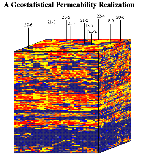
a typical realization for permeability is given in Figure 4. Formation
tops for individual layers were obtained using ordinary kriging.
Numerical Reservoir Modeling
Fine scale realizations of Vsh
,Sw
, N, and permeability were computed at grid nodes whose dimensions
were 200 by 200 by 5 feet (385,875 grid points). Flow simulation
grid point locations had to be reduced to solve the problem
on a workstation in a reasonable amount of time.
In the horizontal plane a decision was made
to stay with the 200 ft by 200 ft block dimensions (the scale
at which geostatistical simulation was done) to keep enough blocks
between infill wells.
Simulator performance was determined to be
acceptable with up to 40,000 grid blocks (a few hours per run),
dictating the level of vertical upscaling. Layers were grouped
to lump high Vsh
content (shaly) intervals reducing the model to 24 layers with
37,800 grid blocks.
Simple upscaling techniques were used for computing
effective permeability of the coarse blocks because the reduction
factor was only about 0.10 and adjacent fine layers of similar
Vsh
properties were grouped together. Vertical permeability was computed
by harmonic averaging with horizontal permeability computed
using arithmetic averaging. Effective porosity of the coarse
blocks was also computed by arithmetic averaging.
There are ten Cotton Valley wells in the simulated
area. Hydraulic fractures were modeled conventionally with increased
permeability near the well blocks using local refined grids. Experiments
with local grids confirmed the necessary level of refinement by
matching analytic solutions. Fracture lengths were obtained by
matching the net pressures observed during the hydraulic fracture
treatments. Several different hydraulic fracture models were used
to estimate xf.
Each of these gave reasonably similar results when the net pressures
were matched.
Gas production data by well was the control
parameter with tubing head pressure (ptf)
used as the matching parameter. Average monthly production was
used. CGU 21-2 has the longest production history and has
an extended pressure buildup. We started to match this drawdown
and buildup performance to obtain reasonable permeability multiplication
factors for the whole reservoir. Two types of permeability modifiers
were used in the history match, global and local. Local permeability
in the refined grid near the well accounted for hydraulic fracturing.
A factor of 0.13 for the overall permeability values (derived
by correlation) gave a very good match for the pressure data of
CGU 21-2. Fracture permeability had to be reduced with time,
indicating possible fracture plugging and/or proppant crushing.
The close match of each of the transient drawdown periods (following
the shut-ins) confirmed the decreasing fracture permeability-width
product.
Figure 5 illustrates the history match of the
CGU 21-2 well. The upper portion of Figure 5 match compares
the flowing tubing pressures calculated from all test points and
the extended pressure buildup with the simulated values of bottom
hole pressure. The measured bottom hole pressure values have
been converted to surface values for comparison with the simulated
values in Fig. 5. The lower portion of the figure compares the
actual flow rates input in the model (primarily based on average
monthly production) and each reported well test. Virtually all
of the discrepancies in the pressure match can be understood by
comparison of the test data and monthly production. On several
occasions following a short shut-in period the test production
data are significantly higher than the monthly average production
used to control the model. For these instances, model pressures
exceed the test values. The accurate reproduction of flowing pressures
following repeated shut-in periods lends confidence to the
reservoir description as well. Test pressures at time 2100-2200
days are characteristic of the well response following a shut-in;
monthly production data do not support this explanation. Several
other small anomalies are present. In each case, the variances
are small and cause us to question the reported test data rather
than the simulator response.
The permeability adjustments (from the log
estimated values) were applied uniformly across the reservoir.
The match of subsequent wells was phenomenal. Essentially no
further data modification was required to match the other nine
wells with acceptable accuracy. Additionally, repeated flowmeter
survey results and measured initial bottom hole pressure values
were reproduced. Initial pressure is a difficult value to measure
in very low permeability wells1.
The most continuous zone is the lower, or Taylor
interval. Initial pressure estimates in this interval have been
made by many methods including:
Prior single- and multiple-well models
were based on much simpler reservoir descriptions. Two basic approaches
have been prevalent. These approximations have been necessary
to match the declining well productivity, predict the pressure
level at infill locations, and match the well transient behavior.
In the most common, the net pay in the upper layers is reduced
away from the wellbore1. This is obviously not meant
to imply an actual reduction laterally, but just poor permeability
connectivity in the upper layers. While the gross sand layers
correlate very well over interwell distances, individual porous
and permeable sand lenses result in significant isolation due
to diagenetic alterations.
A second common technique is to actually reduce
the total net pay but maintain a fixed layer thickness. This
technique has the disadvantages that flowmeter results are not
reproduced and transient behavior is significantly in error.
However, it provides a rapid method for matching the well performance
based on this oversimplified model. It is difficult to justify
the smaller gas-in-place indicated in such models
(compared to volumetric calculations), especially when accounting
for flowmeter data and extended pressure buildups.
CGU 21-2 was shut-in for more than
eighteen months to determine the extent of contribution from the
less permeable layers. Figure 6 compares forecasts made with
two simpler models to the match from the geostatistical reservoir
description and the actual data. Both of the simpler models had
resulted in matches of the well performance. The "multiple
layer" match was a multiple well model with decreasing layer
net thickness in the upper layers. The Taylor sand was represented
by a continuous layer. Well performance and infill pressure values
were matched adequately and required pressure dependent permeability
in the fractures. The "single layer" model was a one-well
model that approximately matched well performance with less total
net pay. These two models result in vastly different expectations
for infill well performance. The multiple layer model implies
larger gas-in-place with the implication that some portion
of the poorly connected pore volumes will be accessible to appropriately
placed infill wells. The single-layer model indicated limited
potential for additional drilling.
This model is not uniquely predictive of infill
well performance because the interconnection of the upper layers
and their spatial distribution is uncertain. Bounds for the
maximum and minimum connectivity cases can be established. The
resulting forecast range of predicted infill well performance
indicates commercial potential for such wells.
The single continuous layer model results in
values of thickness that are too low and requires permeabilities
that are too high. The estimated gas-in-place values
are thus far too low and this model predicts a stabilized pressure
significantly below that predicted by the multiple layer approach.
The actual data demonstrate the inability of
both of the simpler reservoir descriptions to model long term
buildup behavior. The early transient behavior and total gas-in-place
are both reflected in the actual data points (Figure 6). There
is much more energy in the system than either model predicts.
The model based on the geostatistical reservoir description
honors all the pay in the wellbore and accurately reproduces the
long term buildup. This model provides very specific estimates
of infill performance.
The "optimal" fracture length and
well spacing depend on the heterogeneity of the system7,8
as well as economic criteria. Historic well development and well
placement may dictate future optima that are different from (and
generally inferior to) a plan developed much earlier. Unfortunately,
the data to create the necessary reservoir description and well
performance forecasts are not generally available at early times.
Engineering optimization resolves current optimal decisions;
the difference between the economic optimum expected with late-time
data following sub-optimal prior decisions is a measure of
the maximum economic value of obtaining additional data, performing
early-time optimization, etc.
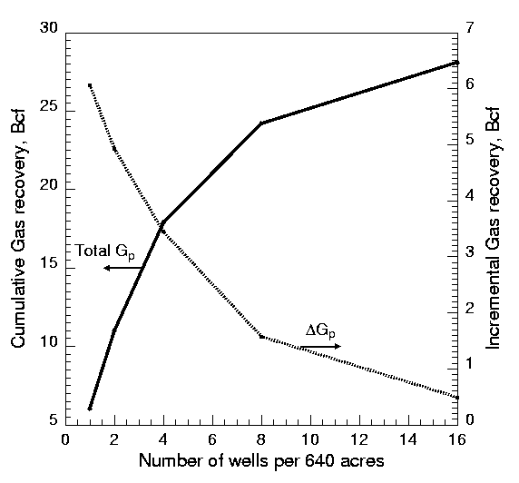
Figure 7 compares the incremental recoveries
predicted by the geostatistical models and multiple layer models
for a typical case (identical fracture lengths). Identical well
performance constraints for each well are used with a maximum
40-year well life. Only the incremental recoveries are given
for these cases; significant acceleration is present for the tighter
spacing. Incremental recoveries are defined as the total incremental
recovery per well comparing one level of spacing with the next.
For example, the total recovery for four 160-acre wells
is 17894.4 MMcf with 24211.2 MMcf for eight wells spaced on 80
acres. The incremental 6316.8 MMcf is allocated to the incremental
four wells for an incremental 1579.2 MMcf per well for 80-acre
spacing. Had all eight wells been drilled initially, each would
average 3026.4 MMcf (according to this model). The actual ultimate
recoveries for 80-acre wells drilled later in time depends
both on when they are drilled and their location. Surface locations
are not always available at a desired spot and prior well locations
may not always have provided for optimal subsequent infill wells.
The wells used to generate the data for Fig. 7 are uniformly
spaced.
The actual economic optimum depends on the
specific location of infill wells, the portion of the field in
which the wells are located and their completion efficiencies.
The geostatistical reservoir description predicts significantly
more incremental recovery for this specific case than does the
multiple layer model. In fact, incremental gas recoveries are
predicted for 40-acre wells!
Unfortunately, the level of incremental recovery
is significantly lower than current economic minimum requirements.
Many Cotton Valley fields have poor recoveries (less than 750
MMcf per well) even for widely spaced wells. In some instances
these areas represent very poor permeability and/or porosity.
Other areas have significant water production. Virtually none
of these areas have been extensively infill drilled in spite of
the fact that they may drain smaller areas than do wells in better
areas.
Further infill drilling and exploitation of
marginal areas depends on improved completions and reduced well
costs. Simple natural gas price increases are often associated
with increased well and leasehold costs. Actually changing the
drilling and completion methodology represents the most important
opportunity to improve the economics of infill drilling and to
improve recovery for low permeability, extremely heterogeneous
reservoirs.
Conclusions
1. A numerical reservoir model for flow simulation was successfully built using geostatistical simulation methods.
2. History-matches of ten wells in the CGU 21 area indicates that hydraulic fracture permeability is reduced with pressure. This indicates that design values of dimensionless fracture conductivity may need to be increased.
3. Accounting for reservoir heterogeneities gives a significantly better match of reservoir performance than do conventional approaches.
4. The geostatistical description of reservoir heterogeneities indicates significant potential for increased recovery from the Cotton Valley interval in Carthage Field.
5. Decreased well costs improve the reservoir recovery efficiency in low permeability, heterogeneous gas reservoirs by increasing the number of commercial infill wells.
Acknowledgments
The authors thank Union Pacific Resources and
the Stanford University Petroleum Recovery Institute (Reservoir
Simulation) for support of this project.
Nomenclature
g(h) Semivariogram
h Vector between attribute pairs
N(h) Number of attribute pairs
xi, yi i-th attribute value
f Porosity
indi Indicator transform level
Vsh Volume fraction shale
Sw Water saturation
wi Weighting factor
V Property estimate
sR Variance
ri Error of the i-th estimate
mR Average error
k Permeability
a a constant
xf Fracture half-length
ptf Flowing tubing pressure
References
1. Meehan, D. N. and Pennington, B. F.: "Numerical Simulation Results in the Carthage (Cotton Valley) Field," paper SPE 9838, Journal of Petroleum Technology, January, 1982.
2. Schell, E. J. : "Drainage Study in the Carthage (Cotton Valley) Field," paper SPE 18264 presented at the 63rd Annual Technical Conference and Exhibition of the Society of Petroleum Engineers held in Houston, TX, Oct. 2--5, 1988.
3. J. Chu, W. Xu, H. Zhu, and Journel, A. G.: "The AMOCO Case Study," July, 1991, Stanford Center for Reservoir Forecasting, Stanford, CA.
4. Deutsch, C. V. and Journel, A. G.:GSLIB: Geoststistical Software Library and User's Guide, Oxford University Press, New York, 1992.
5. Gomez-H., J. and Srivsatava, R.: "ISIM3D: and ANSI-C three-dimensional multiple indicator conditional simulation program," Computers Geosciences, 16(4):395--440,1990.
6. Journel, A. and Zhu, H.: "Integrating Soft Seismic Data: Markov-Bayes updating, and alternative to cokriging and traditional regression," in Report 3, Stanford Center for Reservoir Forecasting, Stanford, CA, May, 1990.
7. Meehan, D.N., Horne, R.N., and Aziz, K.: "The Effects of Reservoir Heterogeneity and Fracture Azimuth on Optimization of Fracture Length and Well Spacing," paper SPE 17606 presented at SPE International Meeting on Petroleum Engineering, Tianjin, China, November, 1988.
8. Meehan, D.N.:Hydraulically Fractured
Wells in Heterogeneous Reservoirs: Interaction, Interference,
and Optimization, Ph.D. Dissertation, Stanford University,
July, 1989.