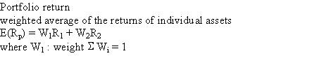
Portfolio Theory
Selection of securities that maximize expected return subject to a level of risk which is acceptable to an investor
Capital Market Theory (CAPM)
Theoretical relationship between risk and return
 

I
Measuring investment return
             V1 – V2 + D
Rp  =   ----------------
                   V0
Where V1 : portfolio MV of the end of the interval
Where V0 : portfolio MV of the beginning of the interval
Where D   : Cash distribution during the interval
 

II
Risky Assets and Risk Free Assets
Future return that will be realized is uncertain
Risk Free asset (riskless)
Short term obligation of US government
 

III
Measuring Portfolio returns and risk
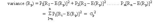
1. Expected portfolio return (mean) – Expected mean
  Quantify the uncertainty about the portfolio  return
  Specify the probability associated with each of possible future returns
        Note : Sum of probabilities = 1
  Given this probability distribution, we can measure the expected return
 
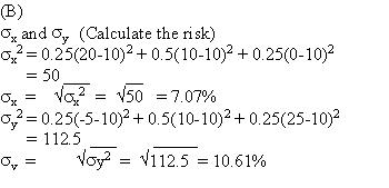
2. Variability of E(Rp)
  measure risk by the dispersion of the possible returns
  measure : variance or standard deviation (weighted sum of the squared deviation from E(Rp) )



 

IV
Diversification
combining stocks into a portfolio to reduce the variance of the returns on your portfolio
while holding returns constant, reduce risk by adding more securities

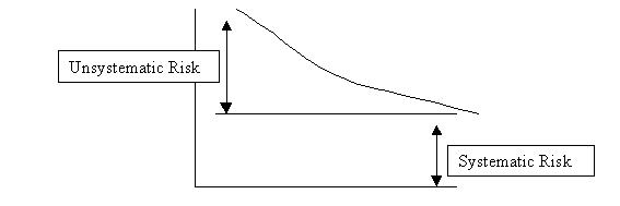
Total Risk
1. Systematic Risk (nondiversifiable risk)
  risk that cannot be eliminated by portfolio combination (market related risk) proxy : S&P 500
2. Unsystematic Risk (diversifiable risk)
  much of the total risk of individual security is diversifiable
  unique to the security

(a) Diversification results from combining securities whose returns are less than perfectly correlated in order to reduce portfolio
     risk
  less correlation ---  greater diversification ---  risk reduced
(b) well diversified portfolio basically carry market risk only.

covariance = how well they move together
correlated may measure linear

cov (x,y) = P1(X1 – E(X))(Y1 - E(Y))
          = P2(X2 – E(X))(Y2 - E(Y))

if cov (X,Y) = 1000
   cov (W,Z) = 500
can’t compare the covariance directly from the number
 

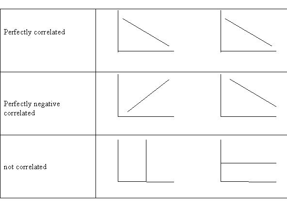
Correlation {-1, 0, +}
p = 1 : perfectly correlated (positively)
p = 0 : not correlated
p = -1 : perfectly negatively correlated
 

EXAMPLE
Portfolio choice
3 state of the world (a, b, c)
two securities (x, y)

State	A	B	C
Probability	0.25	0.5	0.25
x	20%	10%	0%
y	-5%	10%	25%

(A)
Expected Return of X and Y

E(X) = 0.25(20) + 0.5(10) + 0.25(10)
         = 10%
E(Y) = 0.25(-5) + 0.5(10) + 0.25(25)
         = 10%
 

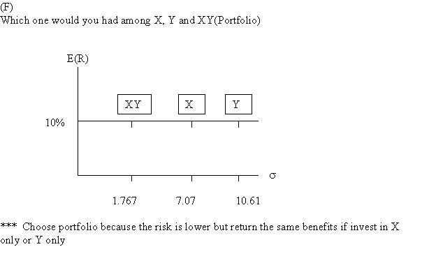
(C )
Portfolio XY formed of one share of X and one share of Y
E(XY) = E(Rp)
            = 0.5(10) + 0.5(10)
           = 10%
 

V
Portfolio Theory
Construction of portfolio that have the highest expected return at a given level of risk
Mean (return) – variance (risk) efficient portfolio ---  Markowitz Efficient portfolio
Assumption
(a) only 2 parameter affect an investor’s decision(mean a variance)
(b) variance are risk averse
(c) investor seek to achieve the highest E(R) at a given level of risk.

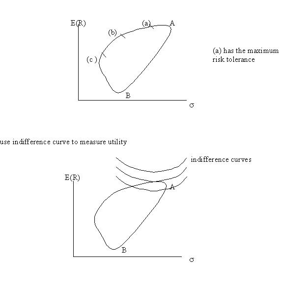
Between point 2 and 4, choose 4 since it return better benefits at the same risks
Point 5 is not real because beyond the efficient frontier
Investor choose any portfolio along the blue line (efficient frontier) that starts from MVP to the tip of the A
 

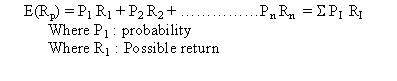
2. Choosing a portfolio in the Markowitz efficient set
investors want to hold one of the portfolio on Markowitz efficient frontier (MEF)
portfolio on MEF ---  trade offs in term of risk and return
Optimal portfolio --- depends on investor’s preference or utility (given investor’s tolerance to risk)