|
........................................ (15 marks)
* Student to participate in discussion and learn spreadsheet terms.
* Students to learn how to enter text, numbers and formulas by following instruction demonstration.
* Students to know the difference between a relative position and an absolute position in a spreadsheet.
* Students to be able to fill a formula down or to the right.
* Students to create and edit a test spreadsheet.
* Students to create a simple chart.
New concepts / terminology:
What is a spreadsheet. -very simply it is rows and columns of numbers that can be calculated very easily. The term comes
from the field of accounting where accountants kept track of business financial activity on large sheets of paper that could
be "spread" out for ease of reading.
The intersection of a row and column is called a cell. There can be millions of cells in a spreadsheet.
You can change the contents of a cell by clicking on the cell and entering information in a space near the top of the
spreadsheet window called the entry bar.
You can work with text, numbers, formulas and logical functions in a spreadsheet.
You can also chart (diagrams or graphs created by the computer) your information.
Lesson 18
1. Open a new Spreadsheet (SS) document and save as "Lesson 18 - Test"
2. Enter column titles in Row 1
a) Move the pointer to cell A1 and click once to select it. Type Name and then the Check Box. The title Name is now
entered in A1. To move to the right use the Tab key
b) Select cell B1 and type Test 1, Tab
c) In Cell C1, type Test 2, Tab
d) In Cell D1, Type Test 3 and then in cell E1, Test 4.
3. Enter the test dates
a) Select cell B2 and type the date 9/12/02. AppleWorks enters and automatically right aligns the date.
b) In cell C2 type in the date 9/26/03, cell D2 10/7/03 and cell E2 10/14/03.
4. Enter the students names
a) Select A3 and type in your name, and then press the Return key. This automatically enters your name into cell A3 and
then moves you down to cell A4.
b) Continue this process by entering the names of 5 other students from your class into cells A4, A5, A6, A7, A8.
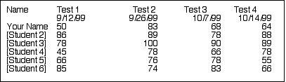
5. Enter the results of the tests.
a) Select cell B3 (opposite your name) and enter the test score of 50. Complete the spreadsheet as shown in the diagram
below:
6. Save the file.
7. Printing a Selected Spreadsheet Area
a) The Set Range command from the Options menu can be used to change the printable spreadsheet area. It is often easier
to first highlight the desired block of cells before executing the Set Print Range.
b) After you have highlighted the range you want to print and have selected the Set Range command from Options, make sure
that the Print Cell Range is selected and the range of cells is also indicated. (eg. To print cells A1 to E8, the range would
look like A1..E8.
c) Print "Lesson 18 - Test" for the first time.
Spreadsheets are a very efficient method to make large calculations using formulas. In order to make the computer know
that you are going to create a calculation you must start your formula with an equal sign (=). Other mathematical operators
are:
...........Brackets....................... ( )
...........Exponentation............. ^
...........Division........................ /
...........Multiplication............... *
...........Addition........................ +
...........Subtraction.................. -
The spreadsheet will calculate using the standard mathematical process called BEDMAS, that is formulas within brackets
first, using exponents, division, multiplication, addition and then subtraction, and then the rest of the formula using the
same order.
As an example, select any empty cell in your spreadsheet and try the following calculations: (remember to start each calculation
with the = sign)
.................. =9+12/3*7 _______
.................. =2*2+3*2 _______
.................. =4+3^2*13 _______
.................. =(6+2)^2 _______
.................. =3+5*6/2*18 _______
.................. =(3+5)*(8+7) _______
.................. =(7+4)*2*22 _______
.................. =25*8/4 _______
Cell names can also be used in formulas. When you have values already entered into cells and want to form calculation,
by entering the cell reference (or by clicking on the cell after you have started with the = sign, the name of the cell appears
BUT the computer will use the value in the cell to complete your calculation.
As an example, select any empty cell in your spreadsheet and try the following calculations: (remember to start each calculation
with the = sign)
In any empty cell enter the value 20 and in the cell to the right enter the value 50. In the next cell to the right enter
the following:
.................. =(click on cell with the value 20)*(click on the cell with the value 50) =_______
.................. =(click on cell with the value 20)+(click on the cell with the value 50) =_______
.................. =(click on cell with the value 20)/(click on the cell with the value 50) =_______
Computers also use functions (words that allow you to make large calculations. The most common are Sum and Average.
Others include Max (for finding the maximum number in a list), Min (minimum number), Round (calculates your answer to a round
number), and PMT (for calculating the payments on loans.)
Other new skills include the use of a special formulas using an absolute cell reference for calculating percentages (when
all numbers in a range are going to be compared to the same number).
Once your spreadsheet has been finished and all of your formulas have been entered, it is also possible to have the computer
show all of your formulas and then print then for future use.
8. Using functions and formulas to calculate Lesson 18 totals, averages.
a) Clear all of the cells that do not have to do with the calculation of your test scores spreadsheet.
b) Move to cell B9 and enter the formula =sum(B3..B8). The value of 410 is displayed.
c) Move to cell B9 and enter the new formula =average(B3..B8). The value of 68.3333333 is displayed.
d) Enter the formulas for the rest of the student to calculate their test averages. Make sure that you change the row
reference to match the students name.
.................. =average(C3..C8) into cell C9
.................. =average(D3..D8) into cell D9
.................. =average(E3..E8) into cell E9
e) Move the cursor to cell F3 and enter the formula =average(B3..E3) and the value 68.25 is displayed as your average
for test score. Repeat the process to calculate the other students test averages.
.................. =average(B4..E4) into cell F4
.................. =average(B5..E5) into cell F5
.................. =average(B6..E6) into cell F6
.................. =average(B7..E7) into cell F7
.................. =average(B8..E8) into cell F8
f) Add a label to cell F1 - Student Average make it bold.
g) Add a label to cell A9 - Test Average make it bold.
h) Right align all of the numbers in your spreadsheet by highlighting the numbers, selecting the Format menu and then
Alignment, select right.
i) Format your Averages to display 1 decimal place by selecting the Format menu and then Number command. Click on Fixed.
Type 1 for the Precision.
Your spreadsheet should look similar to the following:

9. Save your modified Lesson 13 file.
10. ** E-MAIL YOUR "TEST" SPREADSHEET FOR GRADING
Once you feel confident that you have completed this lesson, e-mail your document as an attachment to your instructor
at the following address:
aujla_m@sd36.bc.ca
Your document should include the appropriate file extension in order for the formating to remain in transmission.
For sending documents from Apppleworks, use the extension ".cwk". A correct file name and extension would look
similar to:
L13test.cwk
Notice that any spaces in the file name have been removed and an indicator of which lesson (L13) has been added.
The assigned value for this assignment will be returned once it has been graded.
|